A worked example for one real asset. GeaSpirit uses publicly accessible Earth-observation and geoscience data processed through a proprietary compilation, normalisation, feature-engineering, fusion and interpretation engine. Source provenance is disclosed where appropriate for transparency and technical review; the internal algorithms, transformations, weighting and calibration remain proprietary — two analysts can process the same open data and reach very different results. Illustrative — not a mineral-resource statement.
🔒 PDF download — unlock with your SOST wallet
The PDF is gated. Enter your SOST address; if it holds any amount of SOST (even 0.0001), the download unlocks. Nothing is spent — this only reads your public on-chain balance.
Sample shown for the asset below · the full report is delivered per asset.
◈ Evidence level
—
—
✓ What this report can say
Geological coherence & regional context of the parcel
Surface expression & alteration patterns
Structural setting & open geophysical anomalies
Comparability to known deposit styles
A prioritisation score with an explicit confidence level
✗ What it cannot say
Confirmed grade, tonnage, reserves or resources
Economic viability or recoverability
Ownership, title or legal mining rights
Anything below surface without field validation
A discovery — only field work, sampling & assay can
⛏ Asset
—
—
Asset code
—
Commodity
—
Class
—
Status
—
Coordinates
—
Worked period
—
—/ 100 revival
—
Signal—
Access / depth—
Precision—
Certainty—
How to read the score
Signal
Strength of surface, mineral and geophysical indicators.
Access / depth
Practical recoverability and the likely depth constraint.
Precision
How exactly the evidence overlaps the parcel itself.
Certainty
Confidence given source quality and validation level.
01 Executive summary
—
02 Location, access & setting
Position, terrain and the regional geological belt the asset sits in.
🛰 Surface view
Open optical surface imagery centred on the asset. Location approximate.
📍 Setting
Region
—
Country
—
Geological belt
—
Deposit style
—
Terrain
—
🛣 Access & infrastructure
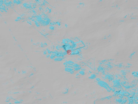
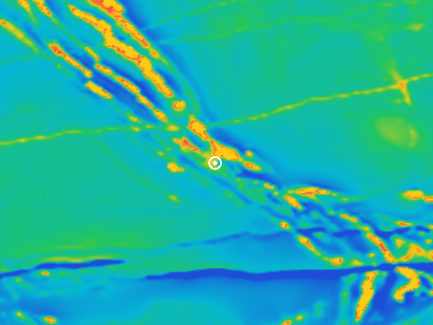
⛰️ Terrain & structural grain
Hillshade from the Copernicus DEM; cyan = strong topographic edges (lineaments). The grain echoes the magnetic structure.
How the exposed ground reflects selected parts of the spectrum — sensitive to iron-bearing, oxidised and disturbed materials. Strong response confirms surface expression; on a known mine it is mostly contextual, and only gains prospective value where it extends beyond the workings.
📖 How to read these — honestly. Warm / bright areas mark a strong surface response from exposed, oxidised or iron-bearing material. On a working or historic mine that response sits largely over the pit, waste rock, haul roads and tailings — so it confirms disturbed, oxidised ground, not remaining ore. The same signal can come from bare soil, dust, processed waste or naturally iron-rich rock. It does not distinguish ore from waste, and does not establish grade or tonnage. Prospective value rises only where a coherent response extends beyond known workings onto undisturbed ground and aligns with structure, geology or an independent data layer.
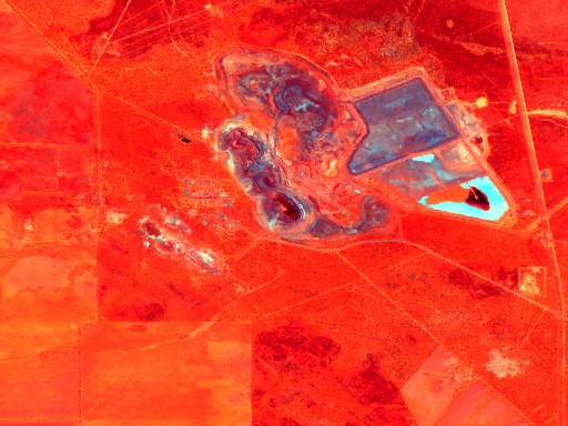
Surface-oxidation spectral composite.These are not natural colours — they are processed differences in the surface's spectral response.Warm red / orange = stronger response from exposed or oxidised material; green = vegetation; blue / cyan often coincides with water or tailings ponds (confirm against the natural-colour view — colour alone does not prove water).lowstrong
What it measures How exposed ground reflects selected spectral bands — sensitive to iron-bearing & oxidised material.
What it shows here Strong response over the pit, disturbed ground & waste — the known mine footprint.
What it may also be Iron-rich soil, bare rock, dust or processed waste — not only mineralisation.
What it does not prove It does not distinguish ore from waste, and gives no grade, tonnage or depth.
Image conclusion: STRONG MINE-RELATED SURFACE RESPONSE — NO EVIDENCE OF REMAINING ORE. Confirms workings, exposed materials & surface oxidation; prospective only where the signal extends beyond the workings.
Provenance: Sentinel-2 surface spectral observation, ~10 m, ESA Copernicus open data. Processed by GeaSpirit (internal indices & transforms proprietary). Sub-metre detail needs commercial imagery; GeaSpirit stays on open sources.
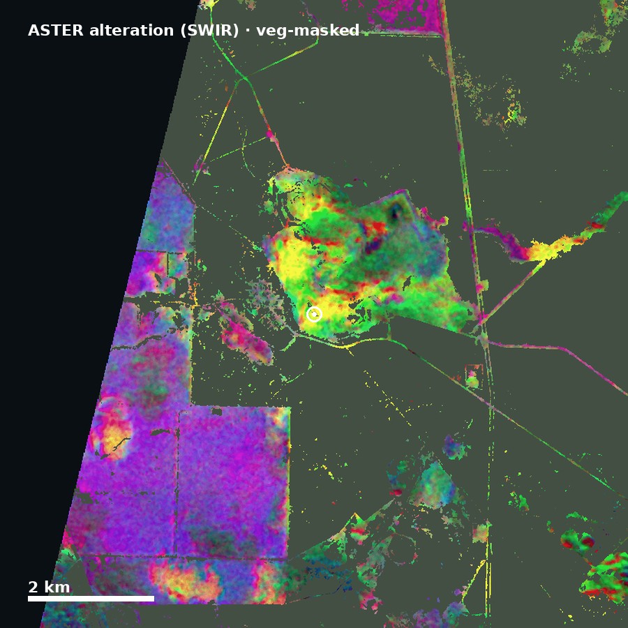
ASTER's SWIR bands (~30 m) resolve clay/mica and chlorite/carbonate absorptions that Sentinel-2 cannot — the hydrothermal alteration minerals that halo around many ore systems. Here as a true alteration-mineral composite, not just "oxidation".
ASTER alteration-mineral composite.SWIR band ratios — not natural colour.R = phyllic / Al-OH (sericite–muscovite–clay, 2.20 µm) · G = propylitic / Mg-OH (chlorite–epidote–carbonate) · B = ferric iron (oxides). Yellow = Al-OH + Mg-OH overlap; neutral grey = vegetation masked out (via Sentinel-2 NDVI, so farmland can't masquerade as alteration); black wedge = edge of the satellite swath (no data).
What it measures Mineral absorptions in the short-wave infrared — the alteration minerals themselves, not just bare/oxidised ground.
What it shows here The asset sits in mildly elevated phyllic (sericite) + propylitic alteration — the halo style expected around orogenic gold.
What it may also be Clay-rich soils, weathering or salt-lake margins can still mimic Al-OH/Mg-OH. Vegetation (≈60% of this scene) is masked out, so it no longer contaminates the read.
What it does not prove Alteration ≠ ore. It gives no grade, tonnage or depth — and here it overlaps the known workings.
Image conclusion: ASSET IN A MILD PHYLLIC + PROPYLITIC ALTERATION CONTEXT — consistent with an orogenic-gold halo, but largely coincident with the known mine. Prospective only where the signature extends onto undisturbed ground.
03× Hyperspectral mineralogy — NASA EMIT
EMIT (NASA imaging spectrometer on the ISS — 285 bands, ~60 m) identifies surface minerals by name from their spectral fingerprint, not by broadband ratio. The strongest free upgrade there is: it confirms the alteration assemblage directly.
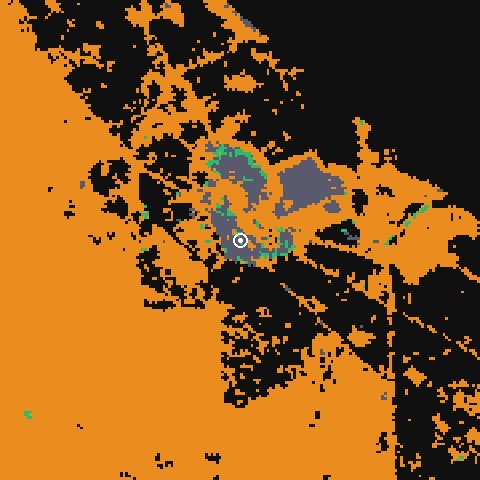
🛰 EMIT mineral map
Orange = iron oxides (goethite/hematite) · green = chlorite/serpentine (mafic/propylitic) · grey = mine footprint / host rock. ~60 m, nearest-neighbour.
🔬 Minerals identified near the asset
📖 Real hyperspectral identification.Chlorite/serpentine (propylitic) + kaolinite/nontronite/vermiculite (argillic clays) + goethite/hematite (iron oxides) + calcite, over weathered greenstone basalt — the alteration assemblage expected around greenstone-hosted orogenic gold. It puts names on what the ASTER ratios only inferred. Band depth = detection strength, not abundance; EMIT's library includes some vegetation/anthropogenic spectra (filtered here); it does not prove gold.
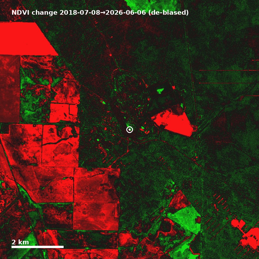
🕓 Surface change — Sentinel-2 (multi-year)
Red = vegetation lost, green = gained, dark = no change. NDVI difference, de-biased by the scene median so only relative change shows (removes the season/year offset).
📊 Change read
📖 NDVI difference between two dry-season images, de-biased by the scene median so a whole-scene wet/dry-year offset cancels and only localised change remains. Red patches over the workings = active mining / clearing; the farmland fields reflect crop cycles; green = regrowth/rehab. It tracks surface disturbance, not ore.
04 Why multi-source — the evidence domains
No single signal is enough. GeaSpirit fuses independent evidence domains; each senses a different physical property of the ground.
🟢
Optical
Surface mapping & oxidation signatures
🟣
Spectral alteration
Clay/hydroxyl hydrothermal footprints
📡
Radar
All-weather structure & surface change
🧲
Geophysics
Intrusions, faults, density/field contrast
⛰️
Terrain & context
Structure, drainage, mining history
Combining independent domains is what turns scattered open signals into a coherent read. The specific sources, weighting and fusion logic are proprietary to GeaSpirit.
05 Open geophysical anomaly maps
Gravity & magnetic anomaly around the asset, from open geoscience data. Steep local contrast marks intrusions, faults and density/susceptibility boundaries — structure that traps & redistributes metal.
lowgravity anomalyhigh
Open free-air gravity field.
lowmagnetic anomalyhigh
Open magnetic anomaly field.
📖 How to read these. Warm colours = high local values, cool = low. A steep change over a short distance (a strong gradient near the asset) marks a geological boundary — an intrusion, fault or contact — and that is exactly where metal tends to concentrate. A flat, uniform field is geologically quiet. The white marker is the asset; white dots are open-data sample points.
06 Geophysical contrast & radar
🎯 Geophysical contrast — local magnetic lead
📡 Radar surface texture
Radar measures surface roughness, geometry & backscatter — not composition. Here the strongest returns correspond mainly to pit benches, embankments, waste areas & mine infrastructure; smooth water or tailings surfaces return darker. It does not identify any mineral or metal.
Image conclusion: clear mining-related surface structure & disturbance — no direct identification of any mineral or metal.
⭕ Circular-structure screening
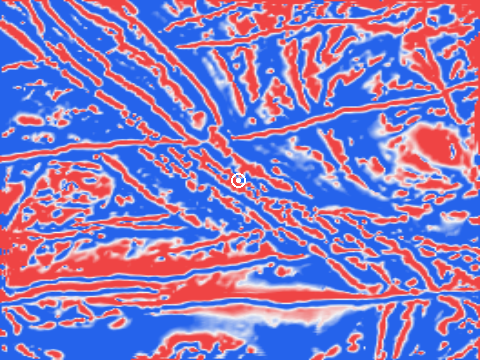
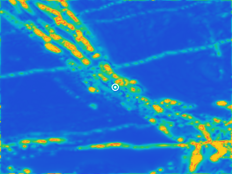
06+ Magnetic field & derivatives — structural read
National high-resolution magnetic grid (Geoscience Australia, ~80 m) processed into structural products. The raw field shows magnetic bodies; the derivatives sharpen edges — contacts, shear zones & dykes — and give a first source-depth estimate.
RTP field (nT). Reduced-to-pole magnetic intensity — highs mark magnetite-bearing units (BIF, mafic / ultramafic rocks).Tilt derivative (°). Normalised edge detector — the linear red/blue grain traces contacts, shears & faults: the structural fabric that channels fluids.Analytic signal. Amplitude of the total gradient — locates magnetic sources regardless of magnetisation direction.
📖 How to read these. The tilt derivative turns the field into structure: its zero line follows geological contacts, and the strong NW–SE grain here is the regional shear fabric of the greenstone belt. The analytic signal peaks over the magnetic bodies themselves — the white marker (asset) sits on a magnetic corridor, the structural setting expected for orogenic gold. The tilt-depth is a first estimate of source depth, not a measurement. This maps structure and magnetic contrast — it does not identify gold or any metal, nor grade, tonnage or depth of ore.
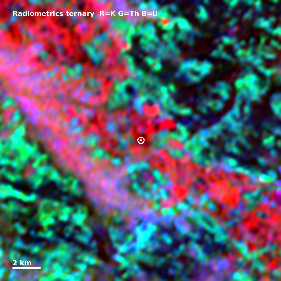
06++ Radiometrics — K / U / Th (gamma-ray)
Airborne gamma-ray spectrometry (Geoscience Australia, ~100 m) maps near-surface potassium, uranium & thorium. Potassium enrichment with low thorium is a classic potassic / sericitic alteration vector for gold.
Ternary K–Th–U. Red = potassium, green = thorium, blue = uranium. The red linear feature through the white marker is a potassium high standing out against the Th/U-rich granitic background.
📖 How to read this. The asset sits on a potassium anomaly (≈0.57 %K vs ~0.20 %K background) with low thorium — added potassium that is not explained by a granite (which would also raise Th). That K-without-Th pattern is the radiometric signature of potassic / sericitic hydrothermal alteration, the alteration style that haloes orogenic gold. It maps near-surface alteration chemistry — it does not prove gold, grade or tonnage, and here overlaps the known workings.
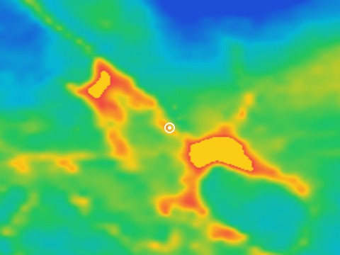
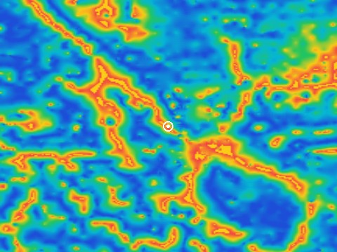
06+++ Regional gravity — density structure
Bouguer gravity (Geoscience Australia, ~400 m) maps subsurface density — dense greenstone belts vs lighter granites. Gold-bearing belts often sit on the density contacts. Regional scale, complementary to the magnetic.
Complete Bouguer anomaly. Highs (warm) = denser crust (greenstone / mafic); lows (cool) = granite.Gravity tilt derivative. Ridges trace density contacts — the granite–greenstone boundaries that channel orogenic gold. The marker sits on a density-contact corridor.
📖 How to read this. The asset sits on a gravity density contact that mirrors the magnetic corridor — independent geophysics pointing at the same structure. Gravity here is regional (~400 m), so it frames the belt-scale setting, not deposit-scale detail. It maps density, not metal — no grade, tonnage or depth of ore.
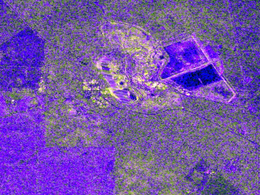
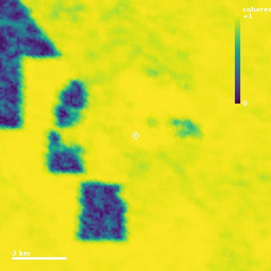
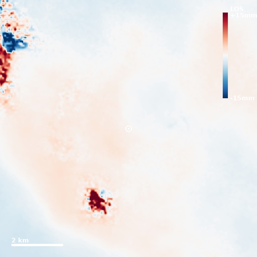
Radar interferometry (Sentinel-1C, recent 12-day pair, processed free via ASF HyP3). Coherence maps surface stability — disturbed/active ground stands out. The displacement is shown detrended (long-wavelength atmospheric/orbital ramp removed) so only relative motion vs the stable surround remains. A single pair screens; sustained mm-scale motion needs a time-series stack.
Coherence (0–1). Green = stable bare ground (high); dark = low coherence over the active mine (disturbance, vegetation, water). The disturbance footprint maps itself.Detrended LOS displacement (12 days, ±15 mm). Ramp removed → red/blue = motion relative to the stable surround. The asset sits near 0 (≈0.6 mm residual): no detectable motion. Localised hot-spots coincide with active pits/tailings. Single pair — a stability check, not a deformation series.
📖 How to read this — honestly. The coherence is the primary product: here it is high (0.89 scene, 0.98 at the asset), confirming a stable arid surface, with the active workings appearing as low-coherence patches — the disturbance footprint maps itself. The displacement is the detrended residual: a single interferogram carries a long-wavelength atmospheric/orbital ramp whose absolute value is meaningless, so we fit and remove that plane and keep only relative motion. The asset's residual is ≈0.6 mm — no detectable ground motion over the 12-day window. This is a stability check, not a deformation measurement: real mm/year subsidence (tailings dams, old workings) needs a time-series stack of many interferograms (a follow-on product). It maps stability and disturbance — not ore.
07 Depth logic
What we can and cannot say about depth — and on what basis. Open-data signals are surface-derived; depth statements must come from documented evidence.
Depth statement
Basis
This asset
Surface signal only
Open surface evidence
✓ available
Depth inferred from deposit model
Geological literature / analogue
model-based
Depth documented
Public drilling / technical report
not attached
Depth confirmed
Field drilling & assay
requires field work
Where this report mentions depth it is inferred from the deposit model, not measured. The satellite/open signal is a surface read.
08 Commodity profile & analogues
⚛ Commodity properties
🌍 Analogue deposit types
Analogue
Type
Note
Reference analogues by deposit style — not a grade/tonnage claim for this asset.
08+ Documented occurrences nearby
Government-recorded mineral occurrences around the asset (Geological Survey of Western Australia, open data). The density of known deposits is one of the strongest first-pass prospectivity signals — and an independent cross-check on the remote-sensing read.
Documented occurrence
Commodity
Distance
📖 How to read this. The asset sits inside a dense gold camp — multiple government-recorded gold occurrences within a few kilometres. This corroborates the magnetic, alteration and radiometric reads with the official deposit record, the kind of independent agreement that lifts confidence. Recorded occurrences are not proof of economic ore on this parcel, and many may be small or worked-out.
09 Red flags & constraints to check
Before any spend, screen these. GeaSpirit flags the categories; confirmation needs local due diligence.
⚠ Environmental protection / protected area⚠ Geological heritage⚠ Urban / residential land⚠ Historical contamination⚠ Permitting status⚠ Access & roads⚠ Water availability⚠ Existing mining rights / overlap⚠ Active project by another party⚠ Community / land tenure
These are checklist prompts, not findings. Each must be verified against local cadastral, environmental and permitting records.
10 Risk & revival thesis
⚠ Key risk factors
♻ Second-chance thesis
—
11 Recommended next actions
A staged, spend-aware path — only advance to the next stage if the previous one justifies it.
Desktop upgrade — pull public technical reports, permits, cadastre & mining history for the parcel.
Field check — site visit, photographs & surface samples to ground-truth the surface signal.
Local geophysics — ground or drone magnetometry / gravity over the anomaly corridor.
Assay — laboratory analysis of representative samples.
Drilling decision — only if the earlier stages justify the cost.
12 Who it is for
Owner
understand whether a parcel has real geological context.
Investor
prioritise & compare assets before committing capital.
Administration
detect sensitive zones, heritage or conflicting use.
Junior miner
filter targets down to a worthwhile shortlist.
Consultant
generate a fast first read before spending on field work.
13 Methodology & provenance
GeaSpirit uses a proprietary multi-source inference workflow combining open Earth-observation data, public geoscience layers and contextual geological information. It evaluates surface expression, alteration patterns, terrain structure, regional geology and mining context to produce an explainable mineral-system coherence read. The specific data stack, transformations, weighting logic and fusion methodology are proprietary to GeaSpirit. The report presents the interpreted result and confidence level, not the internal processing recipe.
Data provenance. The analysis relies on open Earth-observation, geological, cadastral and contextual public datasets. Specific source combinations and processing workflows are proprietary. GeaSpirit provides prioritisation & research intelligence — not a discovery guarantee, valuation, mineral-resource estimate or investment advice.
GeaSpirit reveals the interpreted evidence, not the engine.
Want the full report on this asset?
This is a sample. A full Professional Intelligence Report is generated per asset (or a shortlist), with the complete satellite, alteration, geophysical and structural read, comparables and a revival thesis — delivered in 5–10 days.
Every full report ships with a technical & provenance dossier — every dataset, metric and method used, with sources and units (the full evidence trail). The fusion, weighting and scoring engine stays proprietary; the evidence is documented in full.